Session 03
Numpy - python array computing tool
Brief introduction into numpy and installation
Numpy is a library for the Python programming language, supports large, multi-dimensional arrays and matrices, along with a large collection of high-level mathematical functions to operate on these arrays.
Using Numpy in Python allow the user to write fast programs as long as most operations work on arrays or matrices instead of scalars.
We install the Numpy library directly to our Python IDE.
Open up PyCharm, go to Settings --> Project(name_of_your_project) --> Project Interpreter.
There you should add the required packages by pressing the + symbol and install numpy
from available packages respectively.
If you once installed the pandas library, then the numpy library has already been installed automatically.
Basic steps
Let us implement first simple examples of array creation and basic operations using arrays:
#!/usr/bin/ python
import numpy as np

x = np.array([1,2,3,6])

y = np.arange(10)
# range starts from 0 till 9

z = np.linspace(0,2,4)
# creates an array with four equally spaced elements, starting with 0 and ending with 2

ans = x - z

print("x is equal to: ",x)
print("y is equal to: ",y)
print("z is equal to: ",z)
print("the difference is: ", ans)
We get:
x is equal to:  [1 2 3 6]
y is equal to:  [0 1 2 3 4 5 6 7 8 9]
z is equal to:  [0.         0.66666667 1.33333333 2.        ]
the difference is:  [1.         1.33333333 1.66666667 4.        ]
List comprehensions
List comprehensions is a very important part of Python. It provides a concise way to create lists.
It consists of brackets containing an expression followed by a for clause, then if clauses.
List comprehensions always return a result list.
Let us see some examples regarding list comprehensions.
Before, we used to implement following commands to create a new list from an empty list. We are given a random list of numbers in old_list. We want to create a new_list containing the elements of old_list which are less than 50:
old_list = [88, 13, 28, 51, 19, 63, 92, 27]
new_list = []
for i in old_list:
    if i<50:
        new_list.append(i)

print(new_list)
We get:
[13, 28, 19, 27]
If we use here list comprehensions, we can get a concise form of list:
new_list = [i for i in old_list if i<50]
print(new_list)
We get the same result!
The list comprehensions always starts with square brackets [], reminding you that the result is going to be a list.
The basic syntax is:
[ do something **for** item in list **if** conditional ]
This is equivalent to:
for item in list:
    if conditional:
        do something
Here are some more examples to help you understand it better.
No we will print a range of numbers between 0 and 9 using list comprehensions:
x = [i for i in range(10)]
print(x)

#this will give the output:
[0, 1, 2, 3, 4, 5, 6, 7, 8, 9]
In this example, we are initialising x with seven values and y as an empty list. What we want to do is to fill y with the values of x divided by 5.
The most boring way is:
#! /usr/bin/python
import numpy as np

x = [5, 10, 15, 20, 25, 30, 35]
y = []

for counter in x:
    y.append(counter / 5)
We loop over x and for each value in x we divide it by 5 and add it to y:
print("x = {} \ny = {}" .format(x, y))
The format function in Python has a syntax {}.format(value). Curly braces { } define placeholders, whereas .format(value) returns a formatted string with the value passed as parameter in the placeholder position.
In other words the values to be printed go inside { }, the actual values go inside .format(). We print the values:
x = [5, 10, 15, 20, 25, 30, 35]
y = [1.0, 2.0, 3.0, 4.0, 5.0, 6.0, 7.0]
With the help of list comprehensions, we obtain lighter version of commands:
z = [n/5 for n in x]
print("x = {} \nz = {}" .format(x,z))
We get:
x = [5, 10, 15, 20, 25, 30, 35]
z = [1.0, 2.0, 3.0, 4.0, 5.0, 6.0, 7.0]
If we compare it with the previous example, we see that we have replaced three lines with one line.
Difference between list comprehensions and numpy
Why can’t we just divide x by 5 directly? Let us try it:
try:
   a = x / 5
except:
   print("you can not divide a regular Python list by an integer")
We get:
you can not divide a regular Python list by an integer
This is a try-except block. It tries to run your code and if it finds an exception, it runs the except block.
In this example, you can not divide the list by 5, so it ran the except block.
However, we are able to do this by using numpy arrays. We convert our x array to a numpy array with np.array command:
a = np.array(x)
b = a / 5

print("with numpy: a = {} \nb = {}".format(a, b))
We get:
with numpy: a = [ 5 10 15 20 25 30 35]
b = [1. 2. 3. 4. 5. 6. 7.]
Numpy arrays are sometimes better than list comprehensions. But, we need list comprehensions in many cases. Now you know both ways, so you can choose the best one for yourself.
Plotting sin and cos waves
In this example, we are going to plot a few simple sin and cos graphs, getting an introduction to Python’s plotting library, Matplotlib.
#! /usr/bin/python

import numpy as np
import matplotlib.pyplot as plt
import math
Matplotlib is a huge library. We are using only pyplot part of it.
We are also importing math library. It has many functions that are useful for programs that need to perform mathematical operations.
We use linspace function. As we already implemented before, linspace generates evenly spread out values. We have to generate 1000 values between 0 and 8*pi. Pi is approximately equal to 3.1416.
x = np.linspace(0, 8*math.pi, 1000)
It generates 1000 values which are floating point number by default.
Coming back to our code:
y1 = np.sin(x)
y2 = np.cos(x)

plt.plot(x, y1, "-g", label="sine")
plt.plot(x, y2, "-b", label="cosine")
plt.ylim(-1.5, 1.5)

plt.legend(loc = "upper right")
plt.xlabel("x-axis: 0 to 8*pi")
plt.ylabel("y-axis: -1.5 to 1.5")

plt.show()
We are plotting the graph of the sin function with green color (-g for green) and of the cos function with blue color (-b for blue). We are taking y1 as a function of x for the first graph and y2 as a function of x for the second graph.
We can also set the limits for the y-axis to be between -1.5 and 1.5. By default, it takes between -1.0 and 1.0.
Each function has its own label, sine and cosine. We will show them in the legend, at the upper right side of the graph. You can easily change the orientation of the legend, as you wish.
We can also manually change the labels of x- and y-axis, using .xlabel and .ylabel functions respectively.
We get:
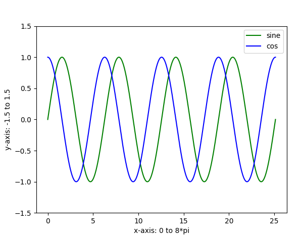
Why are we taking 1000 values for linspace instead of 100? Try it out with 100 and see if it makes a difference.
Plotting salary vs names
In this exercise, we are going to read data from a file and plot it.
All .txt files for this exercise can be found under GIT FH Aachen. Log in with your FH credentials and search for it1-unterlagen. Go to folder Praktikum 3. Download the files and move them directly to that folder where you created your python file.
We have two files: names.txt and salaries.txt. The data in the two files are proportionally linked. So, Jack has a salary of 0, John has 100 and so on.
First we read the salaries:
#! /usr/bin/python

import numpy as np
import matplotlib.pyplot as plt

salary = np.fromfile("salaries.txt", dtype=int, sep=",")
#np.fromfile(file, dtype=float/int, sep="")
By using the np.fromfile() command, we construct an array from the data in a text or binary file.
One of the main features of numpy arrays, that makes them better than normal Python lists is that it allows different types of number data types. Python lists are typically used for strings.
We set datatype argument dtype as int. This tells numpy that datatype is an integer.
The last element is the sep=”,” function, which tells numpy that the data in the file is separated by commas. If the data in the array were seperated by colons, we would use sep=”:”.
We get:
[0 100 200 500 1000 1200 1800 1850 5000 10000]
Now we read the names:
names = np.loadtxt("names.txt",dtype='str',delimiter=",")
#       np.loadtxt(file, dtype=string/float,delimiter="")
The np.fromfile() function does not work with text, so we are using the loadtxt() function. It is similar to the previous function.
Here we set dtype as str. This tells numpy that the datatype is a string.
The last element is the delimiter=”,” function. It does the same as sep() function, but sep is not used to separate string values.
We get:
['Jack' 'John' 'Matt' 'James' 'Sarah' 'Jessica' 'Rupert' 'Pablo' 'Rolanda' 'Bill Gates']
Now we need to plot the names vs salaries. We can not really plot the names on the x-axis, as the x-axis has to be a number.
However, we are able to manage it. The first thing we do is to create a variable x that will contain numbers for each of the names:
x = np.arange(len(names))
The numpy arange generates a list of numbers starting from 0. In our code, x contains a list of numbers from 0 up to the quantity of names.
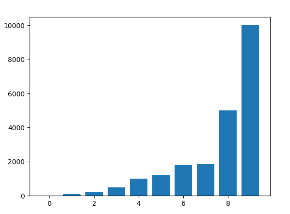
plt.bar(x,salary)
plt.show()
We plot x vs salary. We are using a bar graph here. We get:
We should replace the numbers on the x-axis with actual human names. Because we can only plot against numbers, we had to use this approach.
plt.xticks(x, names)
plt.show()
If one needs to replace names on the y-axis, one should write yticks(). However, in our case, we leave as it is. We get:
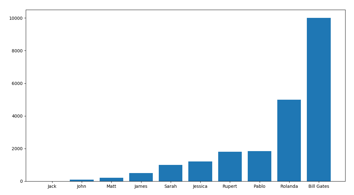
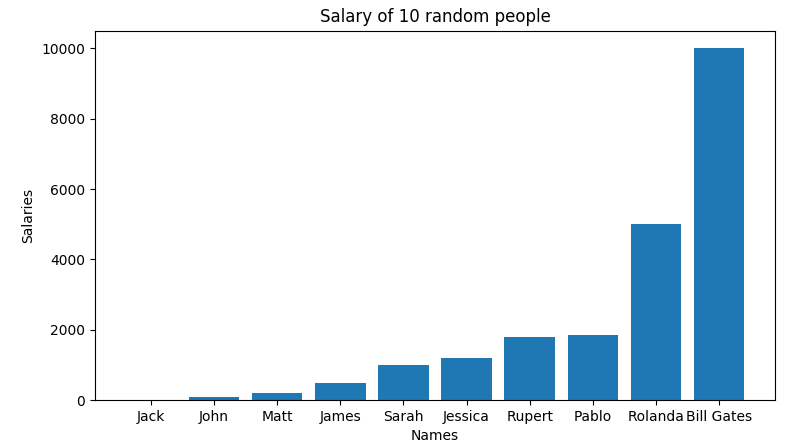
We set x and y labels here. Also we should add a title.
plt.xlabel("Names")
plt.ylabel("Salaries")
plt.title("Salary of 10 random people")
plt.show()
We get a final graph here:
Numpy also supports many functions like maximum, minimum and average values in the array.
max_np = np.max(salary)
min_np = np.min(salary)
aver_np = np.average(salary)

print(max_np, min_np, aver_np)
If we look at the graph above, we realise that the two first and two last values suppress every other values on the background.
Let us modify the graph, so that the graph will illustrate the salaries of people except for Rolanda and Bill Gates.
Before that, we should practice some features of Python:
a = range(5)
# output = [0, 1, 2, 3 ,4]

a[:3]
# output = [0, 1, 2]

a[2:]
# output = [2, 3, 4]

a[2:4]
# output = [2, 3]

a[:-1]
# output = [0, 1, 2, 3]

a[-1:]
# output = [4]
We create a list a that contains values from 0 up to 4 (the last element remains unread).
For a[start value : end value] either the start value or the end value can be empty, in which case it will start at the beginning or go to the end. We can also give both values.
What does -1 mean? Since the list starts at zero, -1 is the last element. -2 is the second last element, and so on.
So, we will use this last trick to get rid of the two first and two last values in our data.
salaries_new = salary[2:-2]
names_new = names[2:-2]

x = np.arange(len(names_new))
plt.bar(x, salaries_new)
plt.xticks(x, names_new)

plt.show()
We get:
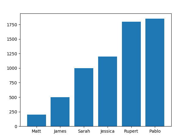
Find the maximum, minimum and average values of a new data by yourself.
Homework
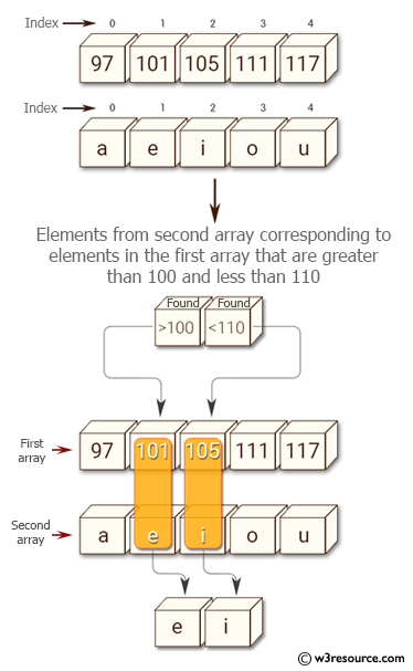
Write a numpy program to select indices satisfying multiple conditions in a numpy array.
Sample arrays:
a = np.array([97, 101, 105, 111, 117])
b = np.array(['a', 'e', 'i', 'o', 'u'])
Select the elements from the second array corresponding to elements in the first array that are greater than 100 and less than 110.
Hint
Check the following image.